Steppi:
An information-based Change-Point Analysis tool for
biophysical applications implemented in MATLAB.
Abstract: Change-point analysis is a flexible and
computationally tractable tool for the analysis of times series
data from systems that transition between discrete states and
whose observables are corrupted by noise. The change-point
algorithm is used to identify the change-points, the times at
which the system transitions between states and fit the model
parameters in each state. We present a unified approach to the
analysis of processes whose noise can be modeled by Gaussian,
Wiener or Ornstein-Uhlenbeck Processes. Using explicit,
closed-form algebraic expressions for maximum-likelihood
estimators of model parameters and estimated information loss of
the generalized noise model that can be computed extremely
efficiently. Next, we demonstrate that a Change-Point Analysis can
be implemented using a single statistical test (Frequentist
Information Criterion) that depends on the number of parameters
fit per state and the number of observations. This approach
reconciles two previously disparate approaches to Change-Point
Analysis (test-statistic and model-selection criterion) for
testing transitions between states. The use of the information
criterion significantly simplifies the statistical analysis and
facilitate the the calculation of explicit expressions for the
resolution of the technique for determining small changes in the
model parameters. We expect this technique to be of general
interest to experimental investigators interested in biological
systems. Applications of this analysis include molecular-motor
stepping, fluorophore bleaching, electrophysiology, particle and
cell tracking, detection of copy number variation by sequencing,
tethered- particle-motion etc.
References: Biophysical Journal
and
Neural Computation.
How change-point analysis works: The change-point
algorithm is used to identify the change-points, the times at
which the system transitions between states and fit the model
parameters in each state. The parameters describing each state are
assumed to be stationary (i.e. not changing in time). The time
evolution of the signal is represented by transitions between the
states. In our biophysical implementation, we parameterize the
state signal with four types of parameters, illustrated in the
figure below:
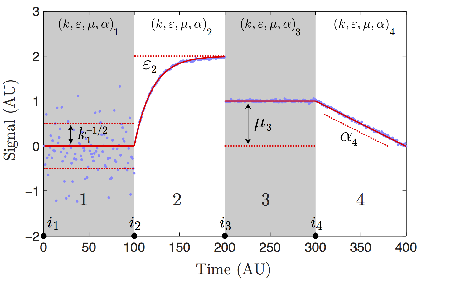
State model schematic. The state model signal is
characterized by four model parameters that are written as the
vector θ ≡ (k, ε, μ, α). Above we schematically illustrate the
role of each parameter in shaping the signal. The parameter k
parameterizes the standard deviation of the noise (σ = k^−1/2).
State two illustrates the effect of the finite lifetime of
fluctuations in models with autoregression (0 < ε < 1).
State three illustrates the role of the level mean μ. State four
illustrates of the role of the level slope (α).
There are three choices for each of these parameters: (i) They may
be set by hand, (ii) They may be chosen to have an unknown but
global value (i.e. shared between all states) or (iii) they may
have an unknown but local value (determined for each state
independently.)
Examples of the Steppi
Package
Download steppi, scripts and data
here.
(1) Wiener Process: Drift Diffusion As an example of a
Wiener Process, we present the example of diffusion with a bias in
one dimension. (The code works in higher dimension as well.) We
simulated data so that the true model is known. The system
transitions back and forth between states with diffusion
coefficients D = { 0.25, 2.5 x 10^-3}/2. The state with the lower
diffusion constant has a small drift velocity with a random
orientation.
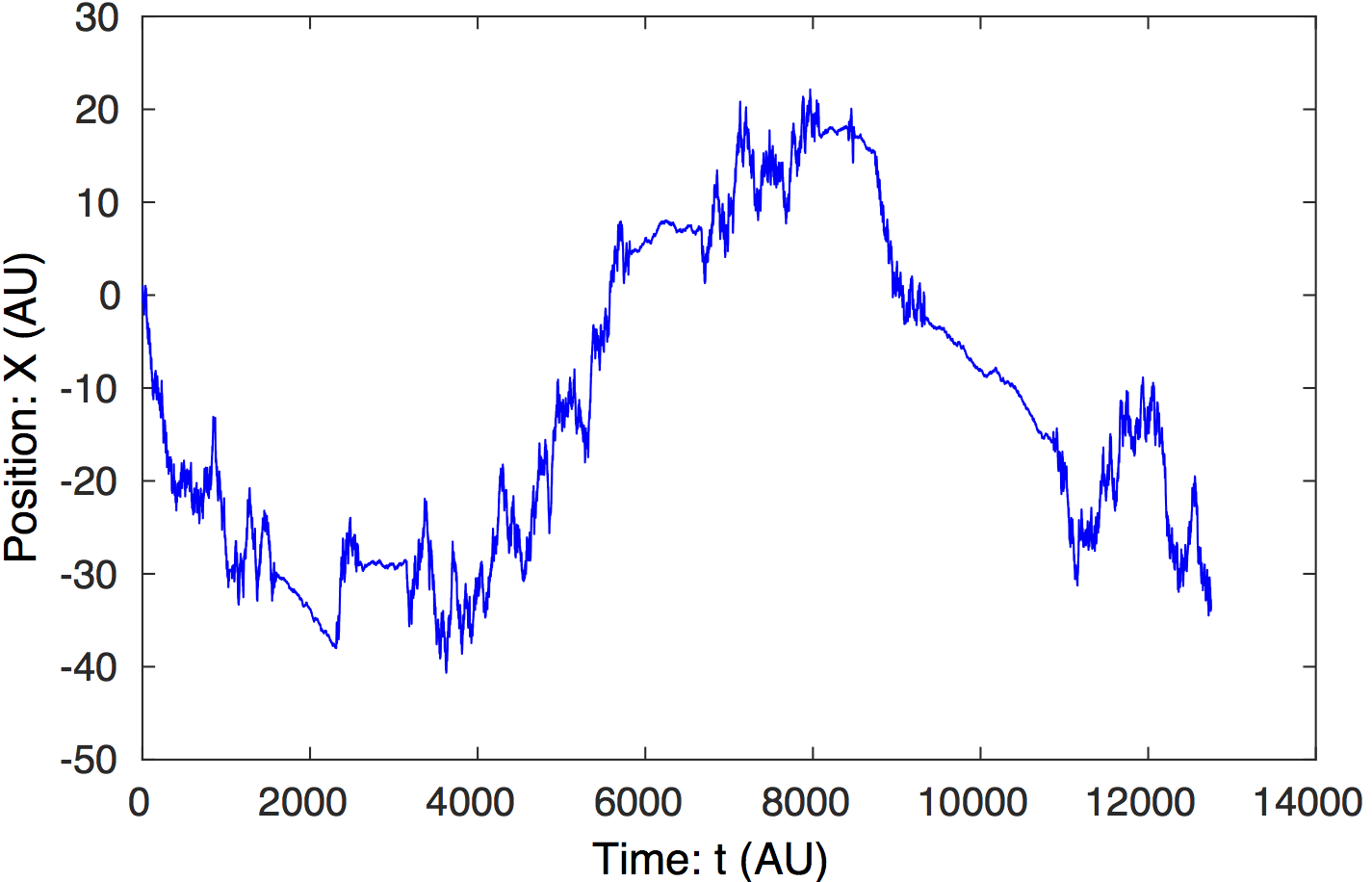
Raw data. The raw particle trajectory
is shown above. The transitions between states with large and
small diffusion coefficients are clearly visible. (E.g. a
transition occurs at t = 1,600.)
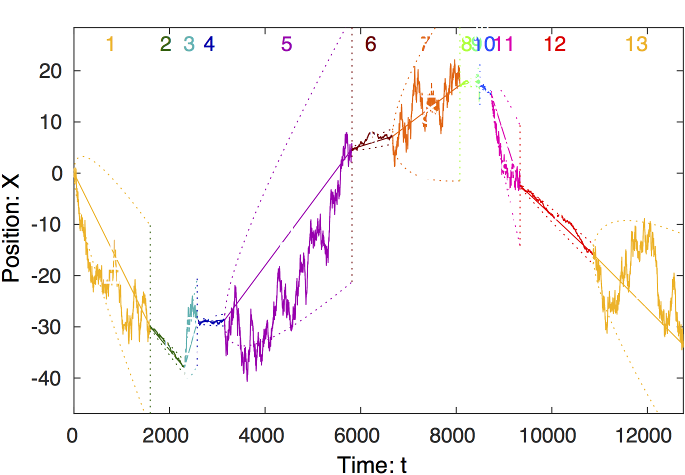
Change-point analysis of signal. Steppi
determines the positions of the change points and fits the
model parameters (a diffusion constant (i.e. stiffness
)
and drift velocity (i.e. level slope
)
in each state. The trajectory is colored by state with the
state number shown at the top of the figure. The true number
of states is recovered (n = 13).
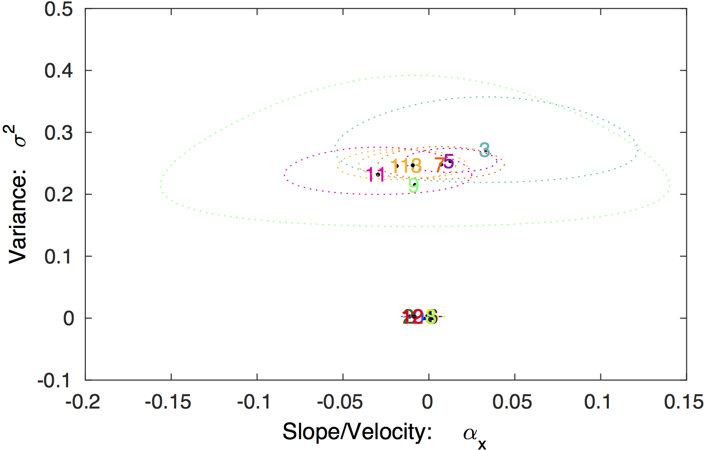
Model parameter values. The 95%
confidence regions for the model parameters for each state is
shown, in addition to the MLE values. The true diffusion
constants are
2D
= { 0.25, 2.5 x 10^-3}, in excellent agreement with the
analysis.
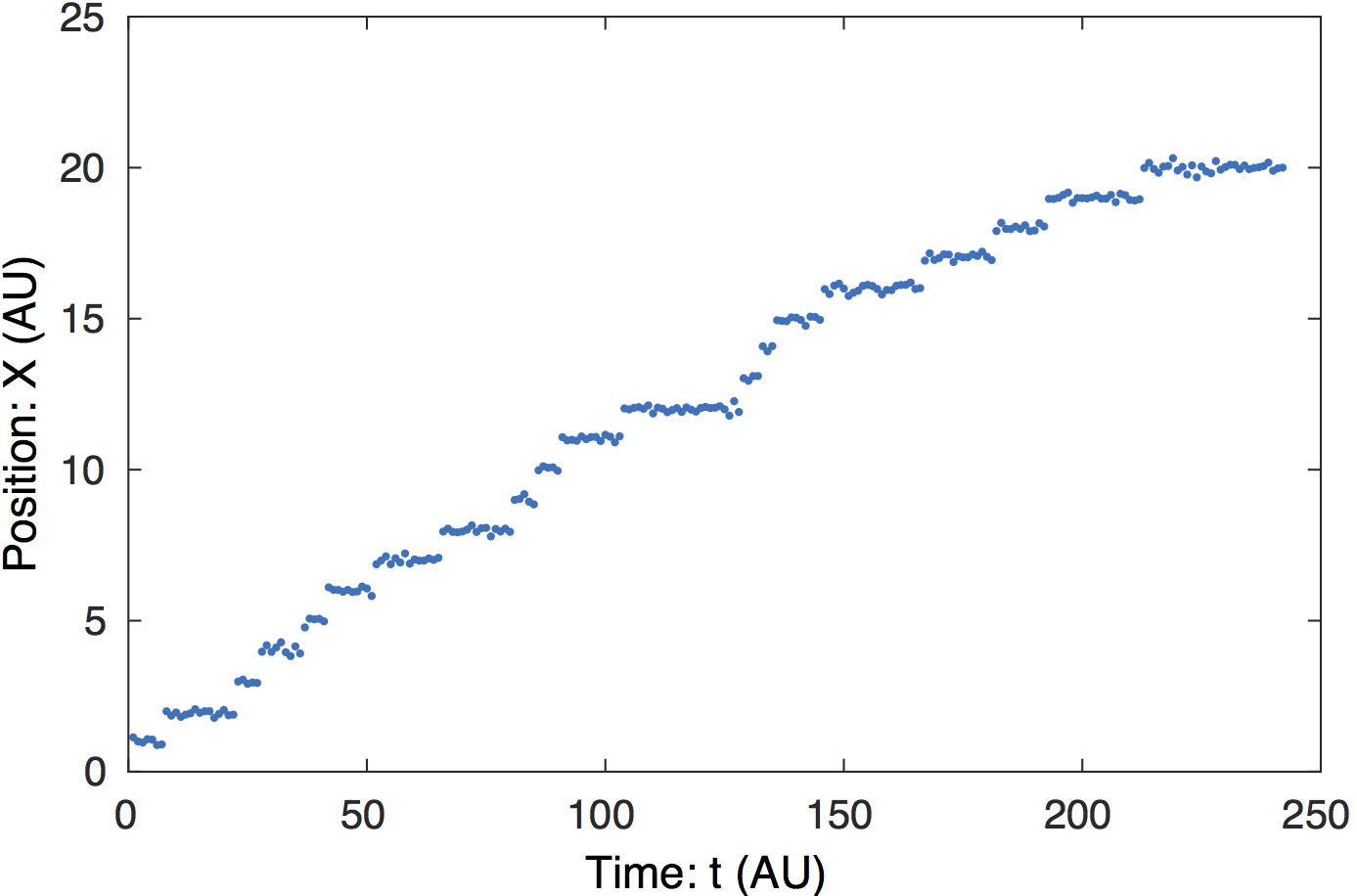
(2) Gaussian Process: Motor stepping
As an example of a Gaussian Process, we present the example of
motor stepping. Again, we simulate the data so that the true
distribution is known. In the change-point analysis, we treat the
motor position as the level mean with an unknown position (unique
for each step) and a global unknown stiffness.
Raw data. In the simulated data, the step length is
1. The step-like transitions are clear by eye.
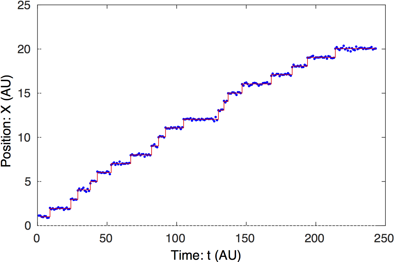
Change-point analysis of signal. Steppi determines the
positions of the change points and fits the model parameters
(level mean
) and
global stiffness (
).
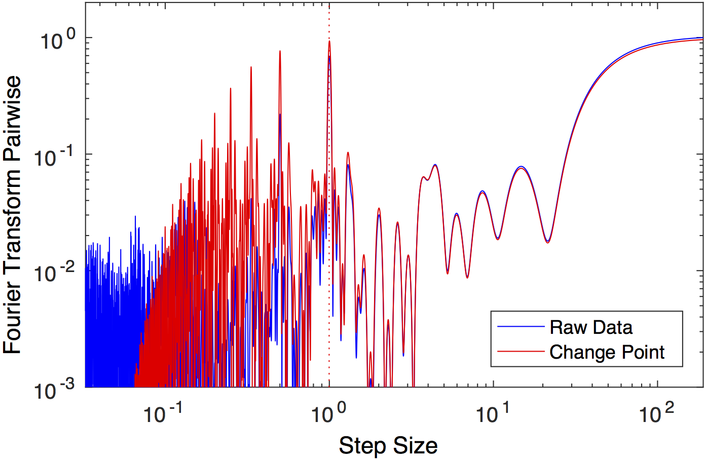
Fourier transform of the pairwise distribution function. A
dotted line shows the peak with the greatest power, corresponding
to the unitary step length, in excellent agreement with the
simulated stepsize 1.
(3) Ornstein-Uhlenbeck Process: Tether Particle Motion
As an example of an Ornstein-Uhlenbeck Process, we present the
example of the analysis of Tethered-Particle-Motion. In short, a
bead diffuses on a a DNA tether. The DNA tether is approximated by
a linear spring. The motion of the bead is therefore subject to
three driving forces: (i) thermal fluctuations, (ii) damping
forces from viscosity and (iii) forces from the deformation of the
DNA tether.
On short time scales, the system behaves like a Wiener Process:
dominated by thermal fluctuations and viscus damping forces. On
long time scales, the system behaves like a Gaussian Process:
dominated by thermal fluctuations and forces from the DNA
tether.
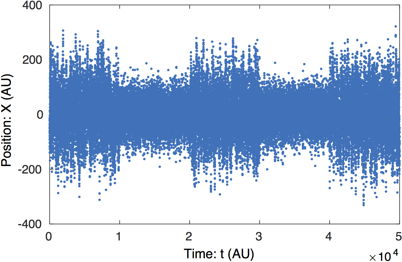
Raw data. Simulated Tethered-Particle-Motion with
short and long tether lengths. The step-like transitions are clear
by eye.
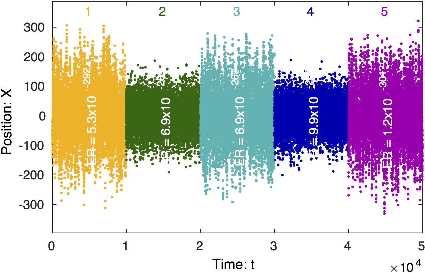
Change-point analysis of signal. Steppi determines the
positions of the change points and fits the model parameters
(level means
),
stiffness (
) and
nearest neighbor coupling (
).
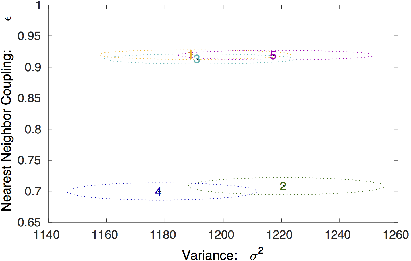
Model parameter values. The 95% confidence regions for the
model parameters for each state is shown, in addition to the MLE
values.