Contents

Clean up everything at the start

clear all
close all hidden
colordef white

% set the defaul size of the windows so they look better on html
set(0, 'DefaultFigurePosition', [100,100,400 ,260]);

Getting help with gateTool commands and syntax

A brief summary of commands and syntax can be found here

help gateTool

  gateTool : tool for gating and plotting functionality of clists.
 
  GATETOOL( [clist,clist cell array,directory,filename], [command string], [argument], ... ) 
  
  clist must be (i) a clist struct or (ii) a cell array of clists or (iii)
  a data directory, xy1 directory or a clist file name. 
 
   If there are no arguments specified, the 'strip' command is run
 
 Clist modification commands:
 
  'merge'      : Merge all clist input into a single output clist (no
                 arguments accepted)
 
  'name', str  : Add name in str to all input clists as a label                 
 
  'color', cc  : Set color cc for all clists
 
  'strip'      : Remove all un-gated cells (no arguments)           
 
  'make', ind  : Gate on indices in ind. Specify either 1 or 2 as a vector 
                 index names are stored in def and can be view by running 
                 the def command. If the ind is a structure it assumes it 
                 is a preformed gate and adds it to the gate array in all 
                 clists. Any gating is performed on all clists input.  
 
  'squeeze'     : make a clist vertical so all entries are treated as
                  identifcal conditions.
 
  'expand'      : make a clist horizontal so all entries are treated as
                  different conditions
 
  'add', data, name : add a field (name) to the clist data with values
                  (data)
 
  'add3D' data, name : add a field (name) to the clist data with values
                  (data)
 
  'get', index  : gets data from data column index  
 %
  'getgate', index : gets the indexed gate.
 
 Visualization commands:
 
  'show', ind   : This command will make a figure for viewing without 
                  modifying the clist. ind is either and index or pair of 
                  indices specifying what is to be visualized. If no ind is 
                  passed then all gates are displayed on a single clist 
                  input         
 
  'kde'         : Make either a 1 or 2D KDE (depending on dimension of ind)
                  'show' must be called as well.
 
  {'time','3D'} : Make a temporal plot of single cell dynamics for one index
                  'show' must be called as well.
 
  'hist'        : Make a 1 or 2D histogram (depending on dimension of ind)
                  'show' must be called as well.   
            
  'dot'         : Make a dot plot. Dim of ind must equal 2.
                  'show' must be called as well.
 
  'line'        :
 
 
  'log', axes   : Set of axes to set with log scales. axes = [1,2,3] will 
                  set x, y and color axis to have log scale.
 
  'den'         : Normalize KDE and hist like a probability density
 
  'cond'        : Normalize like a conditional probability density
 
  'no clear'    : Do not run clear figure (clf) before drawing.
 
  'rk', rk      : radius of the gaussian kernel for KDE
 
  'rm', rm      : radius of the point mask for KDE              
 
  'inv'         : invert 2D hist/KDE image for printing 
 
  'mult', mult  : set the resolution for the KDE. Set the number of pixels
                  in the image created to make ke 
 
  'bin', bin    : set the binning for the hist and KDE. In 1D, if bin is a
                  scalar it is interpretted as the number of bins. If it is
                  a vector it is assumed to be the bin centers. In 2D, if
                  bun is a vector, it is interpretted to be a vector of bin
                  numbers for the two dimensions. If it is a cell array, it
                  is assumed to be two vectors of centers.
 
 
  'err'         : show error in 1D histograms and kde's
 
  'stat'        : show statistics for a show command. Only one index.
 
  'newfig'      : draws new figures for each clist
 
 Other commands:
 
  'def'         : Show all the channel definitions at the command line
 
  'def3D'       : Show all the temporal channel definitions at the command
                  line
 
  'xls', filename : export an excel doc with the clist data. Need to have
                    excel installed to export. (Not my fault.)
 
  'csv', filename, [ind] : export a csv doc with the clist data.
 
  'save', filename : Save .mat file.
 
  'units', units : set the multiplier for the data to set the desired units
 
  'drill'       : Use recursive loading trhough a directory tree to any
                  level.
 
  Copyright (C) 2016 Wiggins Lab
  Written by Paul Wiggins.
  University of Washington, 2016
  This file is part of SuperSegger.
 
  SuperSegger is free software: you can redistribute it and/or modify
  it under the terms of the GNU General Public License as published by
  the Free Software Foundation, either version 3 of the License, or
  (at your option) any later version.
 
  SuperSegger is distributed in the hope that it will be useful,
  but WITHOUT ANY WARRANTY; without even the implied warranty of
  MERCHANTABILITY or FITNESS FOR A PARTICULAR PURPOSE.  See the
  GNU General Public License for more details.
 
  You should have received a copy of the GNU General Public License
  along with SuperSegger.  If not, see <http://www.gnu.org/licenses/>.
 

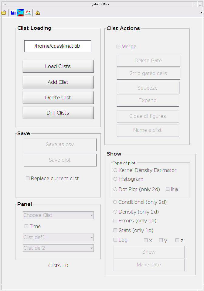
A GUI is available for some gateTool functionality.

gateToolGui

Interactive mode

This flag allows you to either interact with the tutorial by clicking on figures to set gates yourself (by setting the flag to true), or use our predetermined values (interactive_flag = false)

interactive_flag = false;

For a tutorial on using the gateTool function rather than the GUI...

Let's start by loading data, then look at a few helpful examples.

close all hidden

% The data I'll be using is stored in these directories/Clists.
% If you're using the tutorial script rather than the html version,
% change these paths to the path where you have stored the data downloaded
% from the superSeggerWebsite

morph_name   = './Data/morphGating/';
csv_name     = './Data/data.csv';
plasmid_name = './Data/plasmidClist.mat';
ftsZ_name    = './Data/ftsZ/';
growth_name  = './Data/growthClist.mat';
mRNA_name    = './Data/mRNA_clist.mat';

Technical Section: The structure of a clist

Although it is not necessary to understand the implementation, it is often useful since it gives you come understanding of why things are implemented in the way they are. Understanding this section is not required to use gateTool.

% clist (or cell list) is a structure that hold a matrix of cell
% descriptors.

clist = gateTool( mRNA_name, 'add3dt', 'clear' )

% There are two types of data matrices stored in clist: data and data3D
%
% data consists of time-independent descriptors. Each columns represents a
% descriptor and each row a cell
size( clist.data )
% in this case there are 98 decriptors and 20708 cells.
% a descriptor label for each column is stored in the cell array def

% data3D consists of time-dependent descriptors. It is a 3D matric where
% the first index indexes cell, the second indexes descriptors and the
% third the frame
size( clist.data3D )
% a descriptor label is stored in the cell array def3D

% Note that the order of the descriptors is different in data3D and data

% To visualize more than one clist simultaneously, you can construct cell
% arrays of clists. For example let me generate sub-populations of cells
% based on whether cells have old poles or new poles
old_clist = gateTool( clist, ...
                     'gate', 7, [2.1,100],... % select an old pole age
                     ...                      % (index 7) larger than 2 and less than 100
                     'name', 'old cells',...  % label data
                     'color', 'g' );          % select a color
new_clist = gateTool( clist, ...
                     'gate', 7, [0,2.1], ...  % new
                     'name', 'new cells', ...
                     'color', 'b' );
% gates are stored in the gate field
new_clist.gate(1)

% now lets construct a cell array holding both
combo = {old_clist, new_clist};

% gate only foci with good scores
combo = gateTool( combo, 'gate', 12, [4,100], '3d' );

figure(1)
gateTool( combo, 'show', 31, '3d','den' );

Adding field 48: Time (Frames)
Adding field 49: Age (Frames)
Adding field 50: Relative Age

clist = 

         def: {1x98 cell}
        data: [20708x98 double]
      data3D: [20708x50x181 double]
        gate: []
    neighbor: []
       def3D: {1x50 cell}


ans =

       20708          98


ans =

       20708          50         181


ans = 

    ind: 7
      x: [0 2.1000]

How to get your data into gateTool I: clist is already loaded.

There are many ways to get data into gateTool.

% If a clist structure (or cell array of structures) is already loaded, it
% can be passed directly as the 1st argument to gateTool.

% Let's load the data by hand:
pl_clist = load( plasmid_name );

% ... and this data can be passed to gateTool like this.
pl_clist = gateTool( pl_clist );

How to get your data into gateTool II: From a clist.mat file

A clist.mat file can be loaded directly by gateTool The file location is passed to gateTool as the first argument:

pl_clist = gateTool( plasmid_name );

How to get your data into gateTool III: From a superSeger data directory

Since we usually keep clist.mat files in the data directory, gateTool can also load all the clist.mat files (1 for each xy position) saved in a data directory. The directory name is passed as the first argument

morph_clist = gateTool( morph_name );

% a second sloppier option is to recursively load all clist.mat files in a
% directory tree.
morph_clist = gateTool( morph_name, 'drill' );

Loading ./Data/morphGating/xy01/clist.mat
Loading ./Data/morphGating/xy02/clist.mat
Loading ./Data/morphGating/xy03/clist.mat
Loading ./Data/morphGating/xy04/clist.mat
Loading ./Data/morphGating/xy05/clist.mat
Loading ./Data/morphGating/xy06/clist.mat
Loading ./Data/morphGating/xy07/clist.mat
Loading ./Data/morphGating/xy08/clist.mat
Loading ./Data/morphGating/xy09/clist.mat
Loading ./Data/morphGating/xy10/clist.mat
Loading ./Data/morphGating/xy11/clist.mat
Loading ./Data/morphGating/xy12/clist.mat

How to get your data into gateTool IV: From a csv file

There are a couple options to bring in data from other sources (i.e. not superSegger). A csv file can be loaded. The first row is assumed to be the data descriptor names for data in each column.

csv_clist = gateTool( csv_name );

How to get your data into gateTool V: From structures

Another option for bringing in outside data is to use existing structures The descriptor names are copied from the field names.

% lets create some simulated data in two formats
data1 = [];
data1.Area    = rand( [1,100] );
data1.Length  = rand( [1,100] );
data1.Width   = rand( [1,100] );

tmp = [];
tmp.Area   = rand(1);
tmp.Length = rand(1);
tmp.Width  = rand(1);
data2(20) = tmp;

% Both an array of structures and a structure of arrays can be
% automatically converted to the clist format:
data1_clist = gateTool( data1 );
data2_clist = gateTool( data2 );

Trying to convert structure to clist.
Trying to convert structure to clist.

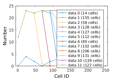
How to label and manipulate data I.

In this first example we demonstrate the typical approach to mani[ulating data, step by step.

% close existing figures.
close all;

% Inputting a directory outputs a cell array of clists from all xy's
clist_all = gateTool( morph_name );

% Note that we will only load the data once. From then on we manipulate the data using the variable clist_all. Check to make sure the data looks ok
% Note that it is necessary always to copy the output of gateTool back into
% a clist variable (clist_all) if you wish to keep the manipulations
% performed by gateTool.
%
figure(1);
clist_all = gateTool( clist_all, 'show', 1 );

% The 'clear' option clears any gates which were previously set during
% segmentation or previous analysis
clist_all = gateTool( clist_all, 'clear' );

% If we have several clists which we would like to treat identically, we
% can use 'squeeze' to treat them as if they were a  single data set. This
% is achieved by making the list of clists vertical (i.e {clist1; clist2}
clist_all = gateTool( clist_all, 'squeeze' );

% One benefit of using 'squeeze' is that it does not actually combine these
% clists into a single clist irreversibly. If we wish to treat all squeezed
% clists as different conditions, we can use 'expand'. This is achieved by
% making the list of clists horizontal (i.e. {clist1, clist})
clist_allExpanded = gateTool( clist_all, 'expand' );

% If in fact we did want to irreverisbly combine the individual clists into
% a single clist, we could use 'merge'
clist_allMerged = gateTool(clist_all, 'merge');

% let's continue with the 'squeeze'd dataset...

% The 'name' and 'color' options allow you to set the future legend label
% and plot coloring any time this clist data is visualized
clist_all = gateTool(clist_all,'name','All Cells','color','k');

% Check to make sure the data looks ok
figure(2);
clist_all = gateTool( clist_all, 'show', 1 );

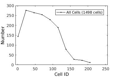
How to label and manipulate data II.

close existing figures.

close all;


% In fact all these steps can be accomplished in a single line:
clist_all = gateTool(morph_name,'clear',...
                     'squeeze','name','All Cells','color','k', ...
                     'show', 1);

What kind of data (descriptors) are in the clist?

%To see what cell characteristics can be visualized, let us check what descriptors have been defined:

close all;

gateTool( clist_all, 'def' );
gateTool( clist_all, 'def3d' );

% wow!

    'Index : Descriptor'
    '1 : Cell ID'
    '2 : Region Num Birth'
    '3 : Region Num Divide'
    '4 : Cell Birth Time'
    '5 : Cell Division Time'
    '6 : Cell Age'
    '7 : Cell Dist to edge'
    '8 : Old Pole Age'
    '9 : Long Axis Birth'
    '10 : Long Axis Divide'
    '11 : stat0'
    '12 : Short Axis Birth'
    '13 : Short Axis Death'
    '14 : Area Birth'
    '15 : Area Death'
    '16 : score birth'
    '17 : score death'
    '18 : x position birth'
    '19 : y position birth'
    '20 : fluor1 sum'
    '21 : fluor1 mean'
    '22 : fluor2 sum'
    '23 : fluor2 mean'
    '24 : number of neighbors'
    '25 : region gray val'
    '26 : locus1_1 longaxis'
    '27 : locus1_1 shortaxis'
    '28 : locus1_1 score'
    '29 : locus1_1 Intensity'
    '30 : locus1_2 longaxis'
    '31 : locus1_2 shortaxis'
    '32 : locus1_2 score'
    '33 : locus1_2 Intensity'
    '34 : locus1_3 longaxis'
    '35 : locus1_3 shortaxis'
    '36 : locus1_3 score'
    '37 : locus1_3 Intensity'
    '38 : locus1_4 longaxis'
    '39 : locus1_4 shortaxis'
    '40 : locus1_4 score'
    '41 : locus1_4 Intensity'
    '42 : locus1_5 longaxis'
    '43 : locus1_5 shortaxis'
    '44 : locus1_5 score'
    '45 : locus1_5 Intensity'
    '46 : neighbors sharing pole'
    '47 : locus1_1_longaxis scale'
    '48 : locus1_2_longaxis scale'
    '49 : locus1_3_longaxis scale'
    '50 : locus1_4_longaxis scale'
    '51 : locus1_5_longaxis scale'
    '52 : locus1_1_shortaxis scale'
    '53 : locus1_2_shortaxis scale'
    '54 : locus1_3_shortaxis scale'
    '55 : locus1_4_shortaxis scale'
    '56 : locus1_5_shortaxis scale'
    '57 : locus1_1_width'
    '58 : locus1_2_width'
    '59 : locus1_3_width'
    '60 : mother ID'
    '61 : daughter1 ID'
    '62 : daughter2 ID'
    '63 : Cum Error Fluor Change Channel 1 (not used)'
    '64 : Cum Error Fluor Change Channel 2 (not used)'
    '65 : Cum Error Shape Spheroplast'
    '66 : Cum Error Fluor Change Channel 1 blind'
    '67 : Cum Error Fluor Change Channel 2 blind'
    '68 : dl max'
    '69 : dl min'
    '70 : l/l_birth'
    '71 : fluor1 sum at death'
    '72 : fluor1 mean at death'
    '73 : fluor2 sum at death'
    '74 : fluor2 mean at death'
    '75 : locus1_1 longaxis at death'
    '76 : locus1_1 shortaxis at death'
    '77 : locus1_1 score at death'
    '78 : locus1_1 Intensity at death'
    '79 : locus1_2 longaxis at death'
    '80 : locus1_2 shortaxis at death'
    '81 : locus1_2 score at death'
    '82 : locus1_2 Intensity at death'
    '83 : locus1_3 longaxis at death'
    '84 : locus1_3 shortaxis at death'
    '85 : locus1_3 score at death'
    '86 : locus1_3 Intensity at death'
    '87 : locus1_4 longaxis at death'
    '88 : locus1_4 shortaxis at death'
    '89 : locus1_4 score at death'
    '90 : locus1_4 Intensity at death'
    '91 : locus1_5 longaxis at death'
    '92 : locus1_5 shortaxis at death'
    '93 : locus1_5 score at death'
    '94 : locus1_5 Intensity at death'
    '95 : locus1_1_width at death'
    '96 : locus1_2_width at death'
    '97 : locus1_3_width at death'
    '98 : long axis / short axis at birth'
    '99 : long axis/ short axis at death'
    '100 : neck width'
    '101 : max width'

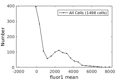
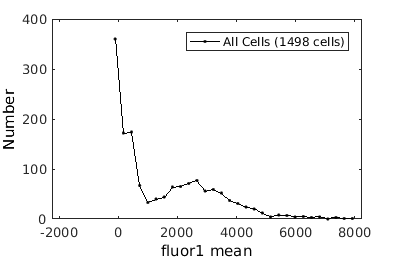
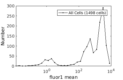
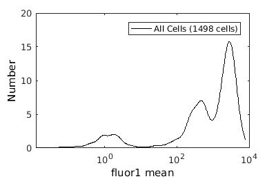
Basic population visualization (1D)

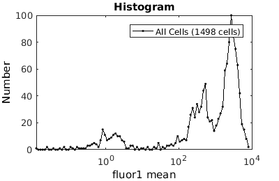
%gateTool has two different visualization options in 1D: histograms and kernel density estimates (kde's).

% close existing figures.
close all;

% Let's look at the fluorescence first, which is index 21.

% First let's use a histogram.
figure(1)
gateTool( clist_all,'show', 21, 'hist' );

% The numer of bins is too conservative so we can set the number by hand.
figure(2)
gateTool( clist_all,'show', 21, 'hist','bin', 30 );

% A log scale is usually better for fluorescence
figure(3)
gateTool( clist_all,'show', 21, 'hist','bin', 30, 'log', 1 );

% Another option is to use the KDE:
figure(4)
gateTool( clist_all,'show', 21, 'kde','bin', 60, 'log', 1 );

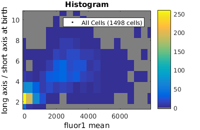
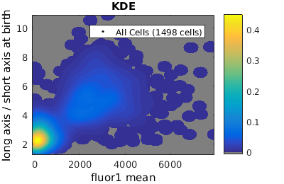
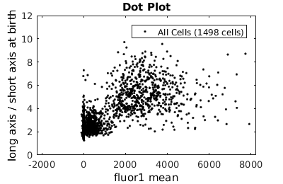
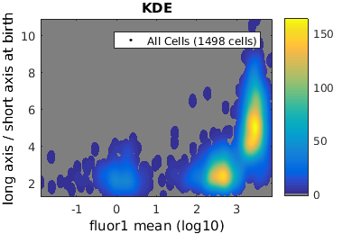
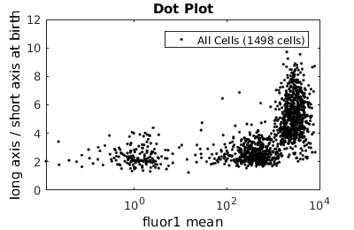
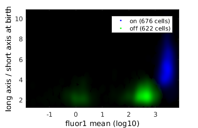
Basic population visualization (2D)

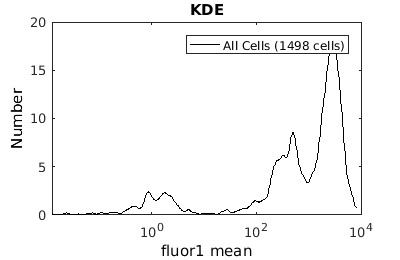
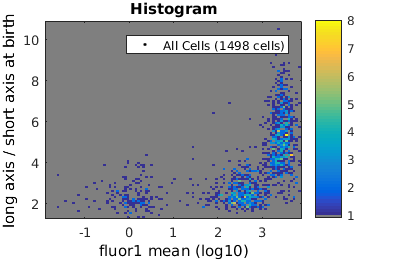
%gateTool has three different visualization options in 2D: histograms, kernel density estimates (kde's), and dot plots.

% close existing figures.
close all;

% Let's look at the fluorescence (21) versus long to short axis ratio (98).
figure(1)
gateTool( clist_all,'show', [21,98], 'hist' );
title( 'Histogram' );

figure(2)
gateTool( clist_all,'show', [21,98], 'kde' );
title( 'KDE' );

figure(3)
gateTool( clist_all,'show', [21,98], 'dot' );
title( 'Dot Plot' );

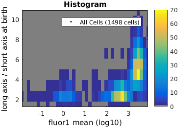
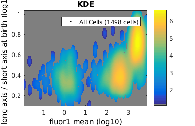
Setting log scale on axes

In some contexts it is convenient to use a log instead of a linear scale on the axis. For example, fluroescence data such as the data plotted in the last section is often better plotted on a log scale. Let's revisit those plots with the x-axis log-scaled.

% close existing figures.
close all;

% Let's look at the fluorescence (21) versus long to short axis ratio (98).
figure(1)
gateTool( clist_all,'show', [21,98], 'hist', 'log', 1 );
title( 'Histogram' );

figure(2)
gateTool( clist_all,'show', [21,98], 'kde', 'log', 1 );
title( 'KDE' );

figure(3)
gateTool( clist_all,'show', [21,98], 'dot', 'log', 1 );
title( 'Dot Plot' );

% The x, y and z (color) axes may all be moved to a log scaling.
figure(4)
gateTool( clist_all,'show', [21,98], 'kde', 'log', [1, 2, 3] );
title( 'KDE' );

Warning: Negative data ignored 
Warning: Negative limits ignored 

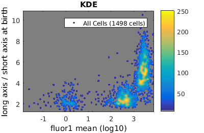
Tweaking the binning and kernel radius by hand

The size of the bins and kde kernel radius are set automatically, but are often not optimal. These can be manipulated by hand.

% In a kde you can supply the radius for each axis in 2D
figure(2)
gateTool( clist_all,'show', [21,98], 'kde', 'log', 1, ...
                                            'rk', [.1,.1] ); % set the radius here
title( 'KDE' );

figure(3)
gateTool( clist_all,'show', [21], 'kde', 'log', 1, 'rk', [.1] );
title( 'KDE' );

% or the number of bins for a histogram
figure(1)
gateTool( clist_all,'show', [21,98], 'hist', 'log', 1, 'bin', [100,100] );
title( 'Histogram' );

figure(4)
gateTool( clist_all,'show', [21], 'hist', 'log', 1, 'bin', [100] );
title( 'Histogram' );

Warning: Negative limits ignored 
Warning: Negative limits ignored 

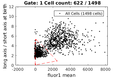
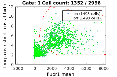
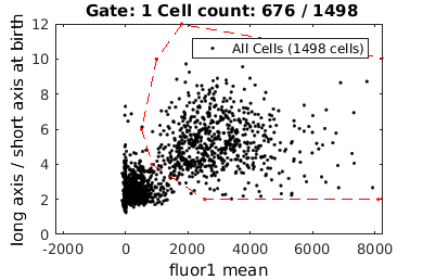
Gating: Defining sub-populations

gateTool allows users to select or gate cells in 1D or 2D.

% close existing figures.
close all;

if interactive_flag
    % Let's gate to cell's whose fluorescence is turned on
    figure(1);
    clist_on = gateTool( clist_all, ...
        'gate', [21,98],  ...
        'log', 1, ...
        'name', 'on', ...
        'color', 'b' );

    % Now, let's gate to cell's whose fluorescence is turned off
    figure(10);
    clist_off = gateTool( clist_all, ...
        'gate', [21,98], ...
        'log', 1, ...
        'name', 'off', ...
        'color', 'g' );

else
    rr = 1.0e+04 *[...
        0.0993    0.0010;...
        0.0514    0.0006;...
        0.0849    0.0004;...
        0.2541    0.0002;...
        0.8103    0.0002;...
        1.1802    0.0004;...
        1.1802    0.0009;...
        0.5064    0.0011;...
        0.1800    0.0012];

    clist_on = gateTool( clist_all, ...
        'gate', [21,98], rr, ...
        'log', 1, ...
        'name', 'on', ...
        'color', 'b' );



    rr = 1.0e+03 *[...
        0.0835    0.0052;...
        1.2361    0.0033;...
        2.4631    0.0009;...
        0.0262    0.0001;...
        0.0001    0.0003;...
        0.0000    0.0015;...
        0.0000    0.0046;...
        0.0001    0.0046;...
        0.0175    0.0052];

    clist_off = gateTool( clist_all, ...
        'gate', [21,98], rr, ...
        'log', 1, ...
        'name', 'off', ...
        'color', 'g' );

end

close existing figures.

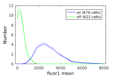
combo = {clist_on, clist_off};

% By inputting a cell array of gated clists, we can view on three clists
% on the same axis, coded by the color/label's we gave each set of data
figure(20);
combo = gateTool(combo, 'show', [21,98], 'log',1, 'kde');

figure(21);
combo = gateTool(combo, 'show', [21], 'hist','err','kde','rk',200);

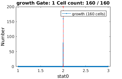
Gating on a single value

For descriptors like stat0, it is convenient to gate a single value. If you supply a single value (rather than a range), the gateTool will only gate on this value (exactly)

% We analyze cell proliferation data. Load data
growth_clist = gateTool( growth_name, ...        % clist filename
                         'name', 'growth', ...   % label the data
                         'clear', ...            % clear any existing gates
                         'gate', 9, 2, ...       % take full cell cycles only
                         'strip', ...            % strip out all ungated data
                         'def3d' );              % show index names for data3D

Full_Cell_Cycle_clist = gateTool(growth_clist, 'gate', 9 ,2 );

    'Index : Descriptor'
    '1 : Cell ID'
    '2 : Long Axis'
    '3 : Short Axis birth'
    '4 : Area birth'
    '5 : fluor1 sum'
    '6 : fluor1 mean'
    '7 : fluor2 sum'
    '8 : fluor2 mean'
    '9 : Number of neighbors'
    '10 : locus1_1 longaxis'
    '11 : locus1_1 shortaxis'
    '12 : locus1_1 score'
    '13 : locus1_1 Intensity'
    '14 : locus1_2 longaxis'
    '15 : locus1_2 shortaxis'
    '16 : locus1_2 score'
    '17 : locus1_2 Intensity'
    '18 : locus1_2 longaxis'
    '19 : locus1_3 shortaxis'
    '20 : locus1_3 score'
    '21 : locus1_3 Intensity'
    '22 : locus1_4 longaxis'
    '23 : locus1_4 shortaxis'
    '24 : locus1_4 score'
    '25 : locus1_4 Intensity'
    '26 : locus1_5 longaxis'
    '27 : locus1_5 shortaxis'
    '28 : locus1_5 score'
    '29 : locus1_5 Intensity'
    '30 : locus_1_1_longaxis pole_align'
    '31 : locus_1_1_longaxis normalized pole_align'
    '32 : locus1_1_longaxis normalized'
    '33 : locus1_2_longaxis normalized'
    '34 : locus1_3_longaxis normalized'
    '35 : locus1_4_longaxis normalized'
    '36 : locus1_5_longaxis normalized'
    '37 : locus1_1_shortaxis normalized'
    '38 : locus1_2_shortaxis normalized'
    '39 : locus1_3_shortaxis normalized'
    '40 : locus1_4_shortaxis normalized'
    '41 : locus1_5_shortaxis normalized'
    '42 : dl max'
    '43 : dl min'
    '44 : l/l_birth'
    '45 : long axis/short axis birth'
    '46 : Neck Width'
    '47 : Maximum Width'
    '48 : Time (Frames)'
    '49 : Age (Frames)'
    '50 : Relative Age'

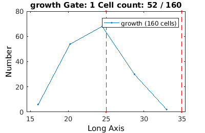
Gating in 1D

Gates in 1D are specified by a range

clist_long = gateTool(growth_clist, 'gate', 10, [25,35]  );

Figuring out what gates have been set

To figure out what gates have been set, you can visualize all the gate

close all;
gateTool( combo, 'show' );

Copying gates between clists

Sometimes one needs to copy gates between structures. We can get the gate out like this

[~,gate_] = gateTool( clist_on{1}, 'getgate', 1);
disp(gate_)

% which we can add to another clist like this:
new_clist = gateTool( clist_all, 'gate', gate_);

    ind: [21 98]
     xx: [9x2 double]

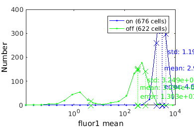
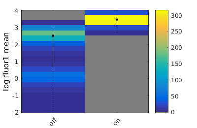
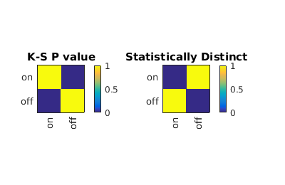
Showing population statistics for different sub-populations

Here we show statistics for each population individually, inluding the KStest statistic for all sup-population pairs. On the left hand side is the p-value and on the right the canonical decision rule.

combo = gateTool(combo, 'show', 21, 'stat', 'log',1);

on -- stats: n = 6.760e+02,  mean: 2.981e+03, std: 1.197e+03, error: 4.603e+01, max: 4.603e+01, min: 4.603e+01.
off -- stats: n = 6.220e+02,  mean: 3.294e+02, std: 3.249e+02, error: 1.303e+01, max: 1.303e+01, min: 1.303e+01.

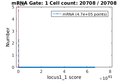
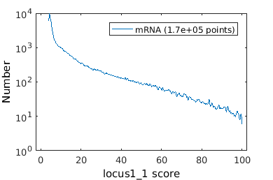
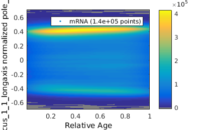
Gating on time-dependent data.

There are many application where one may wish to gate on the time dependent data. Here we will analyze MS2-mRNA complex localization. When superSegger identifies foci, it gives each foci a score which is a proxy for the probability that the focus if real. We therefore wish to get out false positives by putting a floor on the focus score.

% load up mRNA data
mRNA_clist = gateTool( mRNA_name, 'clear',  'name', 'mRNA', 'add3dt', 'def3d');

% Now lets gate on the mRNA focus score
figure(1);
mRNA_clist = gateTool( mRNA_clist, 'gate', 12, [4,100], '3d');
figure(2);
gateTool( mRNA_clist, 'show', 12, '3d' , 'kde', 'log',2);

% Now we show a KDE of focus position
figure(3);
gateTool( mRNA_clist, 'show', [31,37], '3d' , 'kde','rk',[.02,.02]);

% We can also study the population dynamics of the mRNA foci
gateTool( mRNA_clist, 'show', [50,31], '3d' );

Adding field 48: Time (Frames)
Adding field 49: Age (Frames)
Adding field 50: Relative Age
    'Index : Descriptor'
    '1 : Cell ID'
    '2 : Long Axis'
    '3 : Short Axis birth'
    '4 : Area birth'
    '5 : fluor1 sum'
    '6 : fluor1 mean'
    '7 : fluor2 sum'
    '8 : fluor2 mean'
    '9 : Number of neighbors'
    '10 : locus1_1 longaxis'
    '11 : locus1_1 shortaxis'
    '12 : locus1_1 score'
    '13 : locus1_1 Intensity'
    '14 : locus1_2 longaxis'
    '15 : locus1_2 shortaxis'
    '16 : locus1_2 score'
    '17 : locus1_2 Intensity'
    '18 : locus1_2 longaxis'
    '19 : locus1_3 shortaxis'
    '20 : locus1_3 score'
    '21 : locus1_3 Intensity'
    '22 : locus1_4 longaxis'
    '23 : locus1_4 shortaxis'
    '24 : locus1_4 score'
    '25 : locus1_4 Intensity'
    '26 : locus1_5 longaxis'
    '27 : locus1_5 shortaxis'
    '28 : locus1_5 score'
    '29 : locus1_5 Intensity'
    '30 : locus_1_1_longaxis pole_align'
    '31 : locus_1_1_longaxis normalized pole_align'
    '32 : locus1_1_longaxis normalized'
    '33 : locus1_2_longaxis normalized'
    '34 : locus1_3_longaxis normalized'
    '35 : locus1_4_longaxis normalized'
    '36 : locus1_5_longaxis normalized'
    '37 : locus1_1_shortaxis normalized'
    '38 : locus1_2_shortaxis normalized'
    '39 : locus1_3_shortaxis normalized'
    '40 : locus1_4_shortaxis normalized'
    '41 : locus1_5_shortaxis normalized'
    '42 : dl max'
    '43 : dl min'
    '44 : l/l_birth'
    '45 : long axis/short axis birth'
    '46 : Neck Width'
    '47 : Maximum Width'
    '48 : Time (Frames)'
    '49 : Age (Frames)'
    '50 : Relative Age'

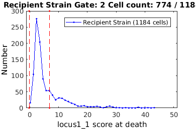
Another Gating Example: Identifying plasmid conjugation through fluorescence gating

% close existing figures.
close all;

% The 'clear' option clears any gates which were previously set
clist = gateTool( plasmid_name, 'clear' );

% The 'name' and 'color' options allow you to set the future legend label
% and plot coloring any time this clist data is visualized
 clist_all = gateTool(clist,'name','All Cells','color','k');

% Gate to donor strain by mean mCherry fluorscence and GFP focus score
if interactive_flag

    clist_ds = gateTool(clist_all, 'gate', [23,28], 'log',1,'log',2, ...
                                'name','Donor Strain','color','g');
else

    rr = [...
        114.1199   59.2553;...
        102.6654   10.2392;...
        102.3041    0.3383;...
        109.3922    0.0260;...
        137.5679    0.0585;...
        145.5516    3.9784;...
        157.8467   46.7830;...
        130.9422   70.1522];

    clist_ds = gateTool(clist_all, 'gate', [23,28], rr,'log',1,'log',2,...
                                   'name','Donor Strain','color','g');
end

% Gate to reipient strain by mean mCherry fluorscence and GFP focus score
if interactive_flag
    clist_rs = gateTool(clist_all, 'gate', [23,28], 'log',1,'log',2,...
        'name','Recipient Strain','color','b');
else
    rr = [...
        175.8974   27.4647;...
        155.2926    6.4856;...
        140.9504    1.6379;...
        144.4067    0.2957;...
        228.8171    0.3058;...
        367.6219    0.3617;...
        372.7464    7.6708;...
        347.8189   98.3357;...
        199.9267   48.5947];
    clist_rs = gateTool(clist_all, 'gate', [23,28],rr, 'log',1,'log',2,...
        'name','Recipient Strain','color','b');
end

% Gate to plasmid recipients by GFP score at division
if interactive_flag
    clist_pr = gateTool(clist_rs, 'gate', 71,...
        'log',2,'name','Plasmid Recieved','color','g');
else
    clist_pr = gateTool(clist_rs, 'gate', 71,[9.2722,47.3770],...
        'log',2,'name','Plasmid Recieved','color','g');
end

% Gate to non-recipients by GFP score at division

%clist_nr = gateTool(clist_rs, 'gate', 71, 'log',2,'name','No Plasmid Received','color','r');
if interactive_flag
    clist_nr = gateTool(clist_rs, 'gate', 71,...
        'log',2,'name','No Plasmid Received','color','b');
else
    clist_nr = gateTool(clist_rs, 'gate', 71,[-0.1996,6.8770],...
        'log',2,'name','No Plasmid Received','color','b');
end

% Use the 'show' option to see all clists and gates
gateTool({clist_all,clist_ds,clist_rs,clist_pr,clist_nr},'show');

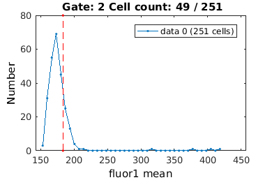
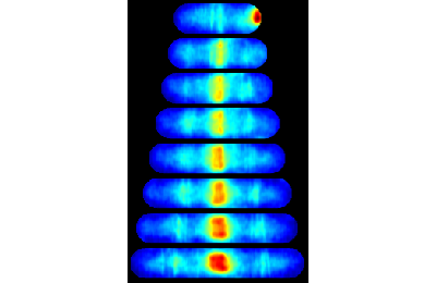
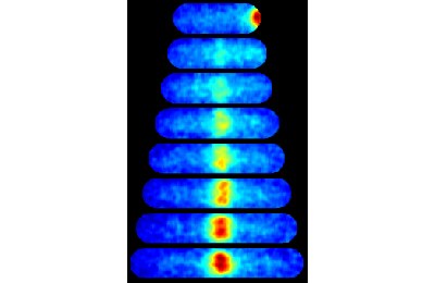
Consensus Example: Visualizing z-ring placement using consensus images

Consensus iamges allow you to see an average of time-lapse fluorescence images. Let's start by looking at a consensus image of FtsZ localization in cells expressing FtsZ at a higher level.

close all;

% Gate to cells with a full cell-cycle observed (i.e. stat0 = 2)
clist_all = gateTool(ftsZ_name,'clear');
if interactive_flag
    clist_ccc = gateTool(clist_all,'gate',11);
else
    clist_ccc = gateTool(clist_all,'gate',11,2);
end

% Gate to highest intensity (using clist 21 'fluor1 mean')
if interactive_flag
    clist_high = gateTool(clist_ccc,'gate',21,...
        'name','High fluor.','color','g');
else
    clist_high = gateTool(clist_ccc,'gate',21, [183.5081,472.3790],...
        'name','High fluor.','color','g');
end
% Load the constants used to segment this data
CONST = load([ftsZ_name,'CONST.mat']);

Make the consensus image

close all

% Display consensus image FtsZ cells gated with high intensity
[ imMosaic, imColor, imBW, imInv, imMosaic10 ] = makeConsensusImage(...
          [ftsZ_name,'cell/'], CONST, 1, 4, false, 1, clist_high );
figure(1);
clf;
imshow(imColor,[]);

Computing consensus array (max cell number 100)

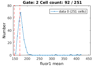
Now let's gate to cells with a lower FtsZ expression level to comapre

close all

% Gate to lowest intensity (using clist 21 'fluor1 mean')
if interactive_flag
    clist_low = gateTool(clist_ccc,'gate',21,...
                        'name','Low fluor.','color','b');
else
        clist_low = gateTool(clist_ccc,'gate',21,[147.3063,170.2289],...
                        'name','Low fluor.','color','b');

end

close all

% Display consensus image of ASKA FtsZ gated with low intensity
[ imMosaic, imColor, imBW, imInv, imMosaic10 ] = makeConsensusImage(...
           [ftsZ_name,'cell/'], CONST, 1, 4, false, 1, clist_low );

figure(2);
clf;
imshow(imColor,[]);

Computing consensus array (max cell number 100)

Use the 'show' option to see all clists and gates

gateTool({clist_all,clist_high,clist_low},'show');

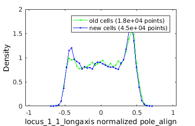
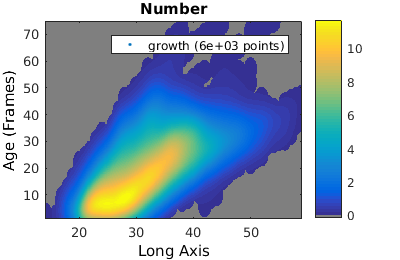
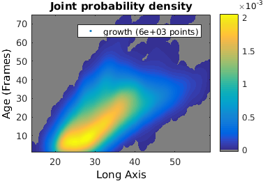
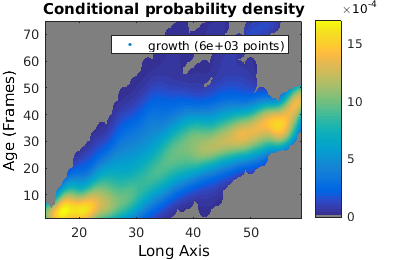
Probability, joint and conditional probability distributions

To compare two populations with different number of individuals it is useful to compare the estimated probability distribution (rather than the histogram).

% We analyze cell proliferation data. Load data
growth_clist = gateTool( growth_name, ...        % clist filename
                         'name', 'growth', ...   % label the data
                         'clear', ...            % clear any existing gates
                         'gate', 9, 2, ...       % take full cell cycles only
                         'strip', ...            % strip out all ungated data
                         'def3d' );              % show index names for data3D

% Show '3D' distribution of cell age versus length
figure(1);
gateTool( growth_clist, 'show', [2,49], '3d' );
title( 'Number' );

% if we want to treat this data as a joint probability density, we plot it as a density
figure(2);
gateTool( growth_clist, 'show', [2,49], '3d', 'den' );
title( 'Joint probability density' );

% We can also generate a conditional probability density
figure(3);
gateTool( growth_clist, 'show', [2,49], '3d', 'den', 'cond' );
title( 'Conditional probability density' );

    'Index : Descriptor'
    '1 : Cell ID'
    '2 : Long Axis'
    '3 : Short Axis birth'
    '4 : Area birth'
    '5 : fluor1 sum'
    '6 : fluor1 mean'
    '7 : fluor2 sum'
    '8 : fluor2 mean'
    '9 : Number of neighbors'
    '10 : locus1_1 longaxis'
    '11 : locus1_1 shortaxis'
    '12 : locus1_1 score'
    '13 : locus1_1 Intensity'
    '14 : locus1_2 longaxis'
    '15 : locus1_2 shortaxis'
    '16 : locus1_2 score'
    '17 : locus1_2 Intensity'
    '18 : locus1_2 longaxis'
    '19 : locus1_3 shortaxis'
    '20 : locus1_3 score'
    '21 : locus1_3 Intensity'
    '22 : locus1_4 longaxis'
    '23 : locus1_4 shortaxis'
    '24 : locus1_4 score'
    '25 : locus1_4 Intensity'
    '26 : locus1_5 longaxis'
    '27 : locus1_5 shortaxis'
    '28 : locus1_5 score'
    '29 : locus1_5 Intensity'
    '30 : locus_1_1_longaxis pole_align'
    '31 : locus_1_1_longaxis normalized pole_align'
    '32 : locus1_1_longaxis normalized'
    '33 : locus1_2_longaxis normalized'
    '34 : locus1_3_longaxis normalized'
    '35 : locus1_4_longaxis normalized'
    '36 : locus1_5_longaxis normalized'
    '37 : locus1_1_shortaxis normalized'
    '38 : locus1_2_shortaxis normalized'
    '39 : locus1_3_shortaxis normalized'
    '40 : locus1_4_shortaxis normalized'
    '41 : locus1_5_shortaxis normalized'
    '42 : dl max'
    '43 : dl min'
    '44 : l/l_birth'
    '45 : long axis/short axis birth'
    '46 : Neck Width'
    '47 : Maximum Width'
    '48 : Time (Frames)'
    '49 : Age (Frames)'
    '50 : Relative Age'

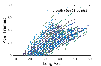
Studying trajectories

We can also construct trajectories

figure(1);
gateTool( growth_clist, 'show', [2,49], ...
                                '3d', ...    % visual time dependent data
                                'dot', ...   % use a dote plot
                                'line' );    % connect the dots

Geting data out of the clist

For some purposes we may want to manipulate the data by hand in matlab. Let's get the cell length at birth and death and the time dependent length out of the clist:

% length at birth
[~,L0] = gateTool( growth_clist, 'get', 10 );

% length at death
[~,L1] = gateTool( growth_clist, 'get', 11 );

% length as a function of time
[~,L ] = gateTool( growth_clist, 'get', 2, '3d' );

% now lets define realtive length
L0_ =  L0*ones([1,size(L,2)]);
L1_ =  L1*ones([1,size(L,2)]);

Lrat = L1./L0;
lam = log(L./L0_)./log(L1_./L0_);

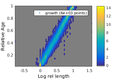
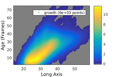
Defining new descriptors

We now wish to add the two new quantities that we have defined to the clist

% add time indep quantity
growth_clist = gateTool( growth_clist, 'add', Lrat, 'Length ratio' );

% add time dependent quantity
growth_clist = gateTool( growth_clist, 'add3d', lam, 'Log rel length' );

% Now show relative age versus relative length
figure(1);
growth_clist = gateTool( growth_clist, 'show', [51,50], 'den', '3d', ...
                         'rk',[.02,.02] ); % modify the kernel radius

% and compare it to age versus length
figure(2);
gateTool( growth_clist, 'show', [2,49], '3d' );

Adding field 99: Length ratio
Adding field 51: Log rel length

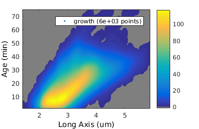
Getting the units correct in figures

All lengths are measured in pixels in superSegger data, but we usually wish to make plots in 'real' units. You can therefore apply a unit conversion factor to put the plots in microns.

% and compare it to age versus length
figure(2);
gateTool( growth_clist, 'show', [2,49], '3d', ...
                         'units', [0.1,1] ); % set the units to 0.1 um
                                             % 3 minute frames
xlabel( 'Long Axis (um)' );
ylabel( 'Age (min)' );

Saving the clist

After loading and manipulating a number of clists, one may want to save the resulting clist (or cell array of clists).

gateTool( growth_clist, 'save', './Data/mod_growth_clist.mat' );

Exporting data to csv format

If you wish to complete your data analysis using software external to matlab, you can save your clist as a csv file.

gateTool( growth_clist, 'csv', './Data/mod_growth_clist.csv' );

Warning: All lists contained in clist will be stripped (ungated data removed) and merged (multiple lists combined) before xls export.

Published with MATLAB® R2016a