| Home | Gene Index | Wiggins Lab |
We present the first proteome-wide characterization of protein localization dynamics. We exploit time-lapse fluorescence microscopy and automated image analysis tools to capture protein localization dynamics throughout the cell cycle in hundreds of single cells for all proteins in E. coli with non-diffuse localization. This approach distinguishes between cell-to-cell variation and cell-cycle dynamics. We compute a distance between all imaged localization patterns, which facilitates the comparison of average protein localization patterns between proteins, including both temporal and spatial structure. Globally, the analysis of these patterns reveals many significant but subtle variations in well established patterns of localization suggesting a large number of mechanisms of protein localization, the majority of which are robust to protein copy number. Finally, we analyze the protein partitioning at cell division and find that in addition to many factors which are retained preferentially in the mother (the cell with the oldest pole) a number of proteins preferentially partition to the daughter. The biological significance of these asymmetries is not yet understood. In addition to the results reported in this paper, we have built a publicly-accessible online database which provides raw and processed data to the research community.
Reference: NJ Kuwada, B Traxler, and PA Wiggins. Genome-scale quantitative characterization of bacterial protein localization dynamics throughout the cell cycle. Molecular Microbiology 95(1):64-79 (2015)
Gene Index
To efficiently categorize the localizome we have organized the strain data into a list of gene names, including synonyms, as defined by the standard ASKA JW-ID. The list is color coded such that strains imaged in this study are in red, strains with existing snapshot data are in blue, and strains without any imaging data (indicating a non-functional fusion) are grey. Clicking on an individual gene name will take you to its Protein Localization Map, which consists of details about the gene, a consensus localization map, and a list of genes with similar spatiotemporal localization patterns. Within the Protein Localization Map, raw images used for analysis can be found in the Single-Cell Data and processed data can be found in the Analysis tab.
Strains. The strains imaged in this collection are predominantly from the ASKA K-12 ORF-clone collection [1], a near complete library of plasmid-based, C-terminal GFPuv4 and N-terminal His-tagged genetic fusions expressed from the IPTG-inducible promoter PT5-lac. Protein localization in this collection has previously been imaged by snapshot analysis [1] and is available online here. For this manuscript we gathered complete cell-cycle time-lapse images of all strains that show non-diffuse localization in the existing snapshot images.
It is important to note that not all of these fusions are functional or show known physiological localization [2,3]. In the cases of proteins where the localization of the ASKA fusion was known to be incorrect or contentious, we supplement the ASKA collection with additional strains from our and/or our colleagues’ collections.
Cell Culture. Cells were inoculated from frozen stock into LB + 34 𝜇g/mL chloramphenicol (Cm34) in a 96-deep-well plate and grown overnight in a 30°C shaker to saturation. The overnight cultures were then diluted 1:40 into M9 minimal media supplemented with Casamino acids (CAA) and Cm34 and allowed to grow for 4 hours, ensuring roughly log phase growth prior to induction. (Detailed Protocol).
Induction of ASKA strains. The expression of the fluorescent fusions in the ASKA collection are IPTG-inducible. Almost all strains were imaged under a least two induction conditions. Strains were induced during log-phase growth in M9 minimal media supplemented with CAA in a 30°C shaker. The following induction conditions are defined accompanied by the approximate protein copy number (inferred from additional single-molecule fluorescence experiments, described in detail below)
| Name | IPTG Concentration (𝜇M) | Induction Time (min) | Protein Number (molecules) |
|---|---|---|---|
| Basal | 0 | 40 | 2x10² |
| 1/10X | 50 | 40 | 2x10³ |
| 1X | 500 | 40 | 2x10⁴ |
Imaging. To image induced cultures, approximately 1-2 𝜇L of cells were pinned from the 96-deep-well induction plate onto a 1.6 mm thick agarose pad supported by a plate-sized glass slide. The pads were sealed on the sides with a rectangular rubber gasket and covered with a large format glass coverslip. For each experiment, 48 cultures were imaged sequentially once every six to eight minutes for 8 hours. The imaging was performed on a Nikon Eclipse Ti-E inverted fluorescence microscope equipped with an environmental chamber (kept at 30°C), a 1.4 NA 60X oil-immersion Ph3 objective, an Andor Neo sCMOS camera, a Nikon Intensilight C-HGFIE, and controlled using the NIS Elements Software package (Advanced Research 4.10). In this microscope configuration, the pixel size was measured to be 0.1079 𝜇m/pixels. Strain positions were visited in a specific pattern to minimize the amount of stage movement between successive points, and auto-focusing at each position prior to image capture was performed using a custom script. Detailed slide preparation and imaging instructions can be found here.
Field of View Data. Raw unprocessed images are directly accessible from the Protein Localization Map for each strain by following the Single Cell Data link. (Currently, only the first frame from the data set is linked.)
Cell Segmentation and Linking. The first step in the analysis of the protein localization is to determine the cell regions (the set of pixels corresponding to each cell in each image) from the phase-contrast image of the culture. Once each frame is segmented, the cell regions are linked between successive frames to make a cell stack, the stack of cell regions, one for each frame during the life of the cell. These image processing steps were carried out using a custom MATLAB software package developed in the Wiggins Lab. (Protocol).
Single-Cell Localization Dynamics. In a typical field of view, we analyzed on order 500 complete cell-cycles. For each dataset in the collection, this single cell data is directly browsable in the form of image towers---see Figure 1---which shows the dynamics localization of the protein SeqA throughout the cell cycle. An image tower corresponds to a stack of images of the cell in successive frames. The first image corresponding to a newborn cell and the last corresponding to the last frame before cell division. To access this data, go to the Protein Localization Map table and click on the Single Cell Data link. The table shows images the first 300 cell analyzed. The raw segmented can be download in a MATLAB mat file linked to each image. (Protocol.)
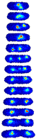 |
| Figure 1: Image tower showing the single-cell localization of SeqA-gfp in false color. The localization in a newborn cell is shown in the first frame. The final frame shows the cell just prior to division. |
Consensus Localization. For almost all proteins with non-diffuse localization there was considerable cell-to-cell variation. To compare localization patterns we therefore needed to develop a method for looking at the average dynamics. We define the consensus localization as the average protein concentration as a function of relative cell position and time relative to the length of the cell cycle. To visualize the data, we again build image towers which shows the consensus localization for the protein SeqA. (Protocol.)
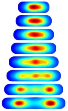 |
| Figure 2: Image tower showing the consensus localization of SeqA-gfp in false color. A consensus image shows the protein concentration as a function of relative cellular position and time relative to the cell cycle. |
Cell-to-Cell Variation Analyzed by PCA. Although the consensus image allows the visualization of the mean protein concentration as function of cellular position and time, the averaging process can obscure important features of the dynamic protein localization pattern. For instance, in the case of MinC, a protein involved in positioning the division plane, the consensus image shows protein localization at both poles but does not capture the characteristic oscillations between poles [4]. To capture repeated patterns in cell-to-cell variation, we use Principal Component Analysis (PCA) which analyzes the correlations between variations spatially and temporally in the cell and weights these patterns by relative occurrence. PCA clearly captures the alternating nature of the MinD oscillation. (Protocol.)
Comparison between consensus localization patterns using a Distance Matrix. The computation of consensus localizations maps facilitates a virtual colocalization measurement: the average dynamic localization of any two proteins can be compared. (It is important to note that since the cell-to-cell average localization is compared, proteins that do colocalize but either do not appear localized in the cell or are not localized to a consistent physical location in the cell will not be detected. For instance, two proteins that form a focus that is not positioned in the cell would not be detected.) To compare localization patterns, we define a distance metric on the localization patterns and then compute of distance metric which represents the distance or difference between any two localization patterns. For each protein, we generate a list of the ten proteins with the most similar localization patterns and place these proteins in the Most Similar Localization Pattern table. Protocol.)
Comparison between consensus localization patterns using PCA. To identify common features between the localization patterns of different proteins, we applied Principal Component Analysis (PCA) to the set of all consensus localization patterns. The Principal Component Vectors represent common modes of variation and can be visualized as images and the Principal Component Loadings reveal the relative importance of these modes of variation. (Protocol.)
Cell Splits Table. To analyze the effect of cell physiology on protein localization, we split our single-cell data into smaller subgroups for further analysis. Because nearly all processes during the cell-cycle are unsynchronized from neighboring cells, e.g. cell length, cell-cycle time, chromosome replication and segregation, etc., a single field of view may contain cells in nearly all stages of the cell-cycle. This, coupled with the fact that we follow cells through multiple division events, allows us to characterize single cell protein localization as a function of many non-trivial cellular characteristics, such as cell length, cell-cycle length, cell birth time, number of cell neighbors, pole age, and total fluorescence, that are not possible in snapshot analysis. We have organized these results for each ASKA fusion the the Cell Splits Table at the bottom of the Analysis page for each strain, and a specific example of Cell Splits analysis can be found here.
Estimating protein copy number by single-molecule imaging. Because the ASKA clones are under an IPTG-inducible promoter rather than their native promoter, the protein expression level is, in most cases, different from the endogenous level. To quantify the amount of protein in the cells for our specific induction conditions, we used high time resolution fluorescence microscopy to observe single-molecule bleaching events [5,6]. By measuring the absolute intensity drop from a single fluorescent protein bleaching event, we can then divide the total integrated fluorescence intensity by the single-molecule intensity to approximate the number of fluorescent proteins within the cell. Approximate protein counts are shown in the table above under 'Induction of ASKA Strains'.
Software Tools.
Custom Autofocus Script (NIS-Elements AR 4.10)
MATLAB Scripts for computing Consensus images, Distance Matrix, PCA, and Asymmetric Partitioning (readme file enclosed).
Data for analysis scripts.
References:
[1] M. Kitagawa, et al. Complete set of ORF clones of Escherichia coli ASKA library (a complete set of E. coli K-12 ORF archive): Unique resources for biological research. DNA Res 12, 291-299 (2005).
[2] M.T. Swulius and G.J. Jensen. The helical MreB cytoskeleton in E. coli MC1000/pLE7 is an artifact of the N-terminal YFP tag. J. Bacteriol. 194(23), 6382-6386 (2012).
[3] D. Landgraf, et al. Segregation of molecules at cell division reveals native protein localization. Nature Methods 9(5): 480-482 (2012).
[4] D.M. Raskin and P.A.J. de Boer. MinDE-dependent pole-to-pole oscillation of division inhibitor MinC in Escherichia coli. J. Bacteriol. 181(20), 6419-6424 (1999).
[5] M. Plank, G.H. Wadhams, M.C. Leake. Millisecond timescale slimfield imaging and automated quantification of single fluorescent protein molecules for use in probing complex biological processes. Integr. Biol. 1, 602 (2009).
[6] R. Reyes-Lamothe, D.J. Sherratt, and M.C. Leake. Stoichiometry and Architecture of Active DNA Replication Machinery in Escherichia coli, Science 328 (5977), 498-501 (2010).